Megatron-LM: Training Multi-Billion Parameter Language Models Using Model Parallelism
摘要 Abstract
近期语言建模方面的工作表明,训练大型 Transformer 模型可以推进自然语言处理(NLP)应用的最先进水平。然而,由于内存限制,非常大的模型可能相当难以训练。在这项工作中,我们介绍了训练超大 Transformer 模型的技术,并实现了一种简单、高效的层内(intra-layer)模型并行方法,使得训练拥有数十亿参数的 Transformer 模型成为可能。我们的方法不需要新的编译器或库的改动,与流水线模型并行正交且互补,并且只需在原生 PyTorch 中插入少量通信操作即可完整实现。我们通过使用 512 块 GPU 训练参数量高达 83 亿的基于 Transformer 的模型并使其收敛来说明这一方法。与单 GPU 的强基线(持续 39 TeraFLOPs,达到峰值 FLOPs 的 30%)相比,我们在整个应用上持续达到 15.1 PetaFLOPs,扩展效率为 76%。为了证明大型语言模型能够进一步推进最先进水平(SOTA),我们训练了一个类似 GPT-2 的 83 亿参数 Transformer 语言模型,以及一个类似 BERT 的 39 亿参数模型。我们表明,随着模型规模增长,在类 BERT 模型中仔细处理 layer normalization 的位置对于获得更好的性能至关重要。使用 GPT-2 模型,我们在 WikiText103(10.8,此前 SOTA 困惑度为 15.8)和 LAMBADA(66.5%,此前 SOTA 准确率为 63.2%)数据集上取得了 SOTA 结果。我们的 BERT 模型在 RACE 数据集上取得了 SOTA 结果(90.9%,此前 SOTA 准确率为 89.4%)。
1 引言 Introduction
自然语言处理(NLP)正在快速发展,部分原因在于可用算力和数据集规模的增长。充足的算力与数据使得通过无监督预训练来训练越来越大的语言模型成为可能(Devlin et al., 2018; Radford et al., 2019)。经验证据表明,更大的语言模型在文章补全、问答和自然语言推断等 NLP 任务上有用得多(Lan et al., 2019; Raffel et al., 2019)。通过在下游自然语言任务上微调这些预训练语言模型,可以取得最先进的结果,近期的工作已表明了这一点(Devlin et al., 2018; Peters et al., 2018; Howard & Ruder, 2018; Radford et al., 2018; 2017; Ramachandran et al., 2016; Liu et al., 2019b; Dai et al., 2019; Yang et al., 2019; Liu et al., 2019a; Lan et al., 2019)。
随着这些模型变大,它们超出了现代处理器的内存上限,需要额外的内存管理技术,例如激活检查点(activation checkpointing)(Chen et al., 2016)。ADAM 等被广泛使用的优化算法为每个参数需要额外的内存来存储动量及其他优化器状态,这降低了能够有效训练的模型规模。若干模型并行方法通过对模型进行划分来克服这一限制,使权重及其相关的优化器状态不必同时驻留在处理器上。例如,GPipe(Huang et al., 2018)和 Mesh-Tensorflow(Shazeer et al., 2018)提供了不同类型的模型并行框架。然而,它们需要重写模型,并且依赖仍在开发中的自定义编译器和框架。
在这项工作中,我们使用层内模型并行实现了一种简单而高效的模型并行方法。我们利用基于 Transformer 的语言模型的固有结构,做出了一个简单的模型并行实现,它可以在 PyTorch 中高效训练,无需任何自定义 C++ 代码或编译器。这一方法与 GPipe(Huang et al., 2018)等所倡导的基于流水线的模型并行正交。
为了展示我们方法的可扩展性,我们建立了一条基线:在单块 NVIDIA V100 32GB GPU 上训练一个 12 亿参数的模型,该模型持续达到 39 TeraFLOPs。这是 DGX-2H 服务器配置下单 GPU 理论峰值 FLOPS 的 30%,因此是一个很强的基线。我们使用 8 路模型并行,在 512 块 GPU 上将模型扩展到 83 亿参数,在整个应用上持续达到最高 15.1 PetaFLOPs 每秒。与单 GPU 情形相比,这是 76% 的扩展效率。图 1 展示了更详细的扩展结果。
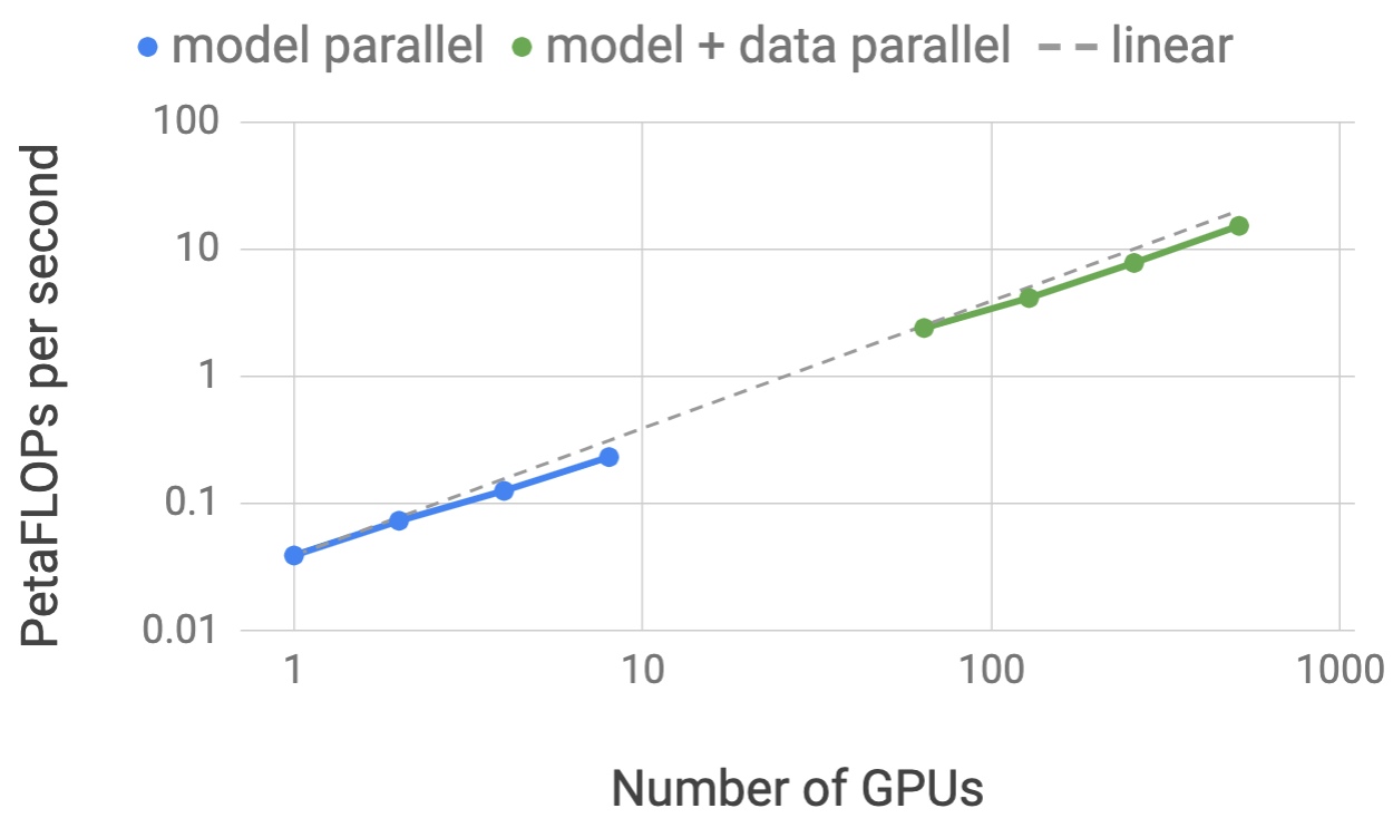
为了分析模型规模扩展对精度的影响,我们训练了从左到右的 GPT-2(Radford et al., 2019)语言模型以及 BERT(Devlin et al., 2018)双向 Transformer,并在若干下游任务上进行评估。我们表明,现有的 BERT 架构会随着规模增大而出现模型退化。我们通过重新排列 Transformer 层中的 layer normalization 与残差连接克服了这一挑战,并表明经过此改动后,下游任务在开发集上的结果随模型规模增大而单调提升。此外,我们表明我们的模型在 WikiText103、LAMBADA 上的完形填空预测准确率以及 RACE 阅读理解数据集上取得了测试集最先进(SOTA)结果。
总结而言,我们的贡献如下:
- 我们仅通过对现有 PyTorch Transformer 实现做少量有针对性的修改,实现了一种简单而高效的模型并行方法。
- 我们对模型并行与数据并行技术进行了深入的实证分析,并证明在使用 512 块 GPU 时可达 76% 的扩展效率。
- 我们表明,随着模型增大,在类 BERT 模型中仔细处理 layer normalization 的位置对于获得更高精度至关重要。
- 我们证明,扩大模型规模可以提升 GPT-2(研究至 83 亿参数)和 BERT(研究至 39 亿参数)模型的精度。
- 我们展示了我们的模型在测试集上取得最先进结果:WikiText103 上的困惑度(10.8 ppl)、LAMBADA 上的准确率(66.5%)以及 RACE 上的准确率(90.9%)。
- 我们开源了代码以及训练与评估流程:https://github.com/NVIDIA/Megatron-LM
2 相关工作 Background and Challenges
2.1 神经语言模型预训练 Neural Language Model Pretraining
预训练语言模型已成为 NLP 研究者工具箱中不可或缺的一部分。利用大规模语料预训练来学习稳健的语言神经表示,是一个跨越过去十年的活跃研究领域。早期的预训练与迁移语言神经表示的例子表明,相比从头学习的词嵌入表,预训练的词嵌入表能够改善下游任务结果(Mikolov et al., 2013; Pennington et al., 2014; Turian et al., 2010)。后来的工作通过学习并迁移能捕获词的上下文表示的神经模型推进了这一领域的研究(Melamud et al., 2016; McCann et al., 2017; Peters et al., 2018; Radford et al., 2017; 2019)。近期的并行工作(Ramachandran et al., 2016; Howard & Ruder, 2018; Radford et al., 2018; Devlin et al., 2018; Liu et al., 2019b; Dai et al., 2019; Yang et al., 2019; Liu et al., 2019a; Lan et al., 2019)在这些想法的基础上更进一步:不仅迁移语言模型以提取上下文词表示,还在下游任务上对语言模型进行端到端的微调。通过这些工作,最先进水平已从仅迁移词嵌入表发展到迁移整个数十亿参数的语言模型。这一方法演进的过程使得我们需要能够在大规模下高效运行并满足日益增长的计算需求的硬件、系统技术和框架。我们的工作旨在提供必要的工具,让这一趋势再向前迈出一步。
2.2 Transformer 语言模型与多头注意力 Transformer Language Models and Multi-Head Attention
由于 Transformer 模型(Vaswani et al., 2017)在精度和计算效率上的优势,当前 NLP 的工作趋向于使用它们。原始的 Transformer 被设计为一种机器翻译架构,使用编码器(Encoder)和解码器(Decoder)两部分,将一个输入序列转换为另一个输出序列。然而,近期利用 Transformer 做语言建模的工作,例如 BERT(Devlin et al., 2018)和 GPT-2(Radford et al., 2019),根据各自需要只使用编码器或解码器。本工作同时探索了解码器架构 GPT-2 和编码器架构 BERT。
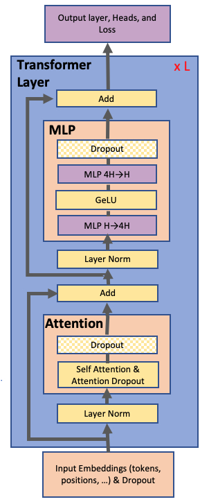
图 2 展示了我们所用模型的示意图。关于模型架构的详细描述,请读者参阅先前的工作(Vaswani et al., 2017; Devlin et al., 2018; Radford et al., 2019)。值得一提的是,GPT-2 和 BERT 都使用 GeLU(Hendrycks & Gimpel, 2016)非线性,并将 layer normalization(Ba et al., 2016)作用于多头注意力层和前馈层的输入,而原始的 Transformer(Vaswani et al., 2017)使用 ReLU 非线性,并将 layer normalization 作用于输出。
2.3 深度学习中的数据并行与模型并行 Data and Model Parallelism in Deep Learning
将深度神经网络训练扩展到众多硬件加速器上有两种核心范式:数据并行(Valiant, 1990),即把一个训练 minibatch 切分到多个 worker 上;以及模型并行,即把模型的内存占用和计算分布到多个 worker 上。通过按可用 worker 数量成比例地增大 minibatch 大小(即弱扩展),可以观察到训练数据吞吐量近乎线性的扩展。然而,大批量训练给优化过程带来了复杂性,可能导致精度下降或收敛时间变长,抵消了训练吞吐量提升带来的好处(Keskar et al., 2017)。进一步的研究(Goyal et al., 2017; You et al., 2017; 2019)发展出了缓解这些影响、缩短大型神经网络训练时间的技术。为了进一步向外扩展训练,并行的工作(Chen et al., 2016)将数据并行与激活检查点结合起来:在反向传播中重新计算激活,而不在前向传播中存储,以降低内存需求。
然而,这些技术在能够处理的问题规模上有一个根本性的限制:模型必须完整地放进单个 worker。随着 BERT 和 GPT-2 这类语言模型的规模和复杂度不断增加,神经网络已经逼近现代硬件加速器的内存容量。解决这一问题的一种办法是采用参数共享来减小模型的内存占用(Lan et al., 2019),但这会限制模型的整体容量。我们的方法是利用模型并行将模型切分到多个加速器上。这不仅缓解了内存压力,还能够独立于 microbatch 大小来增加并行度。
在模型并行内部,还有两种范式:逐层的流水线并行,以及更一般的分布式张量计算。在流水线模型并行中,一组操作先在一个设备上执行,然后其输出被传递给流水线中的下一个设备,由其执行另一组不同的操作。一些方法(Harlap et al., 2018; Chen et al., 2018)将参数服务器(Li et al., 2014)与流水线并行结合使用。但是它们存在不一致性问题。TensorFlow 的 GPipe 框架(Huang et al., 2018)通过使用同步梯度下降克服了这一不一致性问题。这种方法需要额外的逻辑来处理这些通信与计算操作的高效流水化,并且会受到流水线气泡(pipeline bubbles)降低效率的影响,或者需要改动优化器本身,从而影响精度。
分布式张量计算是一种正交且更一般的方法,它把一个张量操作划分到多个设备上,以加速计算或增加模型规模。FlexFlow(Jia et al., 2018)是一个编排此类并行计算的深度学习框架,它提供了一种选择最佳并行化策略的方法。最近,Mesh-TensorFlow(Shazeer et al., 2018)引入了一种在 TensorFlow(Abadi et al., 2015)中指定一类通用分布式张量计算的语言。并行维度由终端用户在该语言中指定,生成的计算图会用恰当的集合通信原语进行编译。我们利用了与 Mesh-TensorFlow 类似的见解,借助 Transformer 注意力头计算中的并行性来并行化我们的 Transformer 模型。然而,我们不是实现一个模型并行的框架和编译器,而是仅对现有的 PyTorch Transformer 实现做少量有针对性的修改。我们的方法很简单,不需要任何新的编译器或代码重写,只需插入若干简单的原语即可完整实现,下一节将对此进行描述。
3 模型并行 Transformer Model Parallel Transformers
我们利用 Transformer 网络的结构,通过添加少量同步原语来创建一个简单的模型并行实现。如图 2 所示,一个 Transformer 层由一个自注意力块以及随后的两层多层感知机(MLP)组成。我们分别在这两个块中引入模型并行。
我们先详细介绍 MLP 块。该块的第一部分是一个 GEMM,后接一个 GeLU 非线性:
$$Y = \mathrm{GeLU}(XA) \tag{1}$$并行化该 GEMM 的一种选择是沿行切分权重矩阵 $A$,并沿列切分输入 $X$:
$$X = [X_1,\, X_2],\qquad A = \begin{bmatrix} A_1 \\ A_2 \end{bmatrix}. \tag{2}$$这种划分将得到 $Y = \mathrm{GeLU}(X_1A_1 + X_2A_2)$。由于 GeLU 是非线性函数,$\mathrm{GeLU}(X_1A_1 + X_2A_2) \neq \mathrm{GeLU}(X_1A_1) + \mathrm{GeLU}(X_2A_2)$,因此这种方法需要在 GeLU 函数之前设置一个同步点。
另一种选择是沿列切分 $A$,即 $A = [A_1,\, A_2]$。这种划分使得 GeLU 非线性可以独立地作用于每个被划分的 GEMM 的输出:
$$[Y_1,\, Y_2] = [\mathrm{GeLU}(XA_1),\, \mathrm{GeLU}(XA_2)] \tag{3}$$这样做的好处是去掉了一个同步点。因此,我们以这种列并行(column parallel)方式划分第一个 GEMM,并沿行切分第二个 GEMM,使其直接接收 GeLU 层的输出而无需任何通信,如图 3a 所示。第二个 GEMM 的输出随后在各 GPU 之间进行规约(reduce),再传给 dropout 层。这种方法将 MLP 块中的两个 GEMM 都切分到各 GPU 上,并且在前向传播中只需要一次 all-reduce 操作($g$ 算子),在反向传播中也只需要一次 all-reduce 操作($f$ 算子)。这两个算子互为共轭,只需几行代码即可在 PyTorch 中实现。作为示例,下面给出 $f$ 算子的实现:
class f(torch.autograd.Function):
    def forward(ctx, x):
        return x
    def backward(ctx, gradient):
        all_reduce(gradient)
        return gradient
Code 1. $f$ 算子的实现。$g$ 与 $f$ 类似,只是在反向函数中为恒等操作,在前向函数中为 all-reduce。
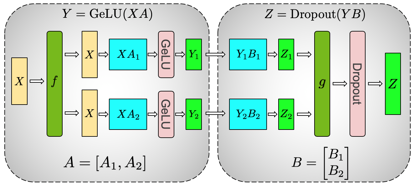
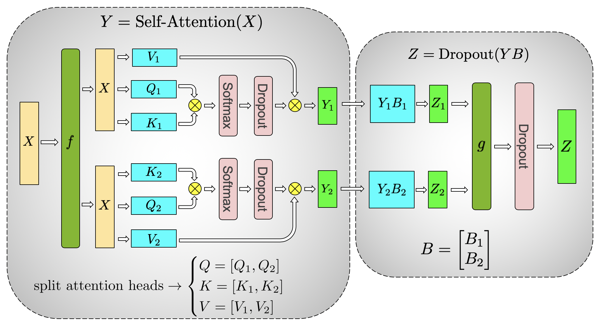
如图 3b 所示,对于自注意力块,我们利用多头注意力操作中固有的并行性,以列并行的方式划分与键(K)、查询(Q)和值(V)相关的 GEMM,使得每个注意力头对应的矩阵乘法都在一块 GPU 上本地完成。这使我们能够把每个注意力头的参数和工作负载拆分到各 GPU 上,并且完成自注意力不需要任何中间通信。随后来自输出线性层(位于自注意力之后)的 GEMM 沿行并行化,直接接收并行注意力层的输出,GPU 之间无需通信。对 MLP 和自注意力层都采用这种做法,融合了成组的两个 GEMM,消除了中间的同步点,并带来更好的扩展性。这使我们能够在一个简单的 Transformer 层中,仅用前向路径中的两次 all-reduce 和反向路径中的两次 all-reduce 完成所有 GEMM(见图 4)。
Transformer 语言模型的输出嵌入的维度为隐藏维度($H$)乘以词表大小($v$)。由于现代语言模型的词表大小在数万个 token 的量级(例如 GPT-2 使用的词表大小为 50,257),并行化输出嵌入的 GEMM 是有益的。然而,在 Transformer 语言模型中,输出嵌入层与输入嵌入共享权重,这需要对二者都进行修改。我们沿词表维度对输入嵌入权重矩阵 $E_{H\times v}$ 进行并行化,即按列切分 $E = [E_1,\, E_2]$。由于现在每个分区只包含嵌入表的一部分,在输入嵌入之后需要一次 all-reduce($g$ 算子)。对于输出嵌入,一种做法是执行并行 GEMM $[Y_1,\, Y_2] = [XE_1,\, XE_2]$ 以得到 logits,再加一次 all-gather $Y = \text{all-gather}([Y_1,\, Y_2])$,并把结果送入交叉熵损失函数。然而,在这种情况下,all-gather 要通信 $b \times s \times v$ 个元素($b$ 是批大小,$s$ 是序列长度),由于词表很大,这个数量非常庞大。为了减小通信量,我们把并行 GEMM 的输出 $[Y_1,\, Y_2]$ 与交叉熵损失融合,使维度降为 $b \times s$。通信标量损失而不是 logits,是通信量的巨大削减,这提高了我们模型并行方法的效率。
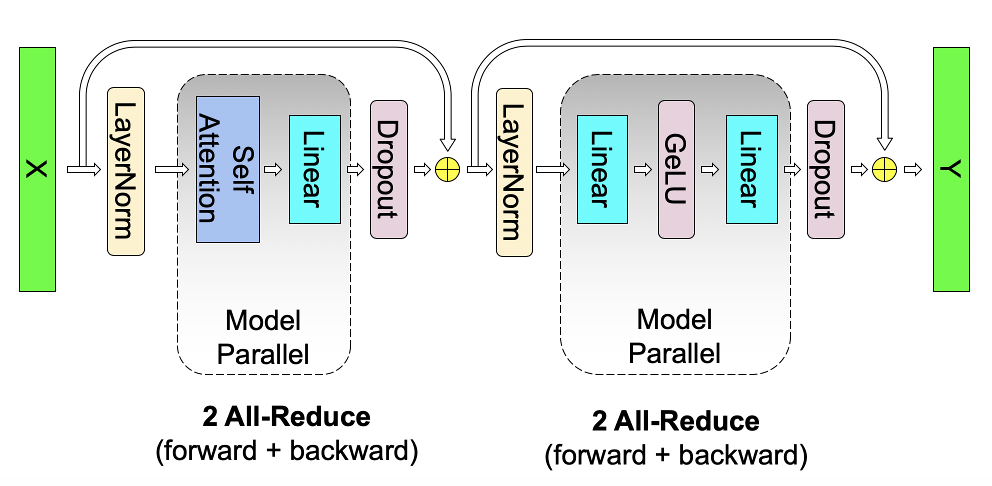
我们的模型并行方法在很大程度上可以概括为旨在减少通信并让 GPU 保持计算受限(compute bound)的技术。我们没有让一块 GPU 计算 dropout、layer normalization 或残差连接的一部分再把结果广播给其他 GPU,而是选择在各 GPU 之间复制这部分计算。具体而言,我们在每块 GPU 上保留 layer normalization 参数的副本,取模型并行区域的输出,在这些张量上运行 dropout 和残差连接,然后再将它们作为输入送入下一个模型并行区域。为了优化模型,我们允许每个模型并行 worker 优化它自己的那组参数。由于所有值要么是 GPU 本地的,要么在 GPU 上被复制,因此在这种方案下无需通信更新后的参数值。
关于混合模型并行与数据并行以及随机数生成的处理,更多细节见附录 B。总之,如上所述,我们的方法实现简单,只需在前向和反向传播中额外加入少量 all-reduce 操作。它不需要编译器,并且与 (Huang et al., 2018) 等方法所倡导的流水线模型并行正交且互补。
4 实验设置 Setup
预训练语言理解模型是自然语言处理和语言理解中的核心任务。语言建模有若干种表述方式。在这项工作中,我们关注 GPT-2(Radford et al., 2019),一种从左到右的基于 Transformer 的生成式语言模型;以及 BERT(Devlin et al., 2018),一种基于语言模型掩码(masking)的双向 Transformer 模型。我们在下文中说明这些模型的配置,更多细节请参阅原论文。
4.1 训练数据集 Training Dataset
为了收集一个具有长程依赖的大型多样化训练集,我们聚合了若干最大的语言建模数据集。我们构建了一个聚合数据集,包含 Wikipedia(Devlin et al., 2018)、CC-Stories(Trinh & Le, 2018)、RealNews(Zellers et al., 2019)和 OpenWebtext(Radford et al., 2019)。为避免训练集泄漏到下游任务中,我们移除了出现在 WikiText103 测试集中的 Wikipedia 文章(Merity et al., 2016)。我们还移除了 CC-Stories 语料中由预处理伪影引入的不必要换行符。对于 BERT 模型,我们在训练数据集中加入了 BooksCorpus(Zhu et al., 2015);但由于该数据集与 LAMBADA 任务有重叠,GPT-2 训练中排除了它。
我们合并了所有数据集,然后从聚合数据集中过滤掉内容长度少于 128 个 token 的所有文档。由于相似的内容可能在聚合数据集中多次出现,我们使用局部敏感哈希(LSH)对 Jaccard 相似度大于 0.7 的内容进行去重。最终得到的聚合语料包含 174 GB 去重后的文本。
4.2 训练优化与超参数 Training Optimization and Hyperparameters
为了高效训练模型,我们采用带动态损失缩放(dynamic loss scaling)的混合精度训练,以利用 V100 的 Tensor Core(Micikevicius et al., 2017; NVIDIA, 2018)。我们首先用简单的正态分布 $W \sim \mathcal{N}(0,\, 0.02)$ 初始化权重 $W$。然后,我们在残差层之前立即用 $\dfrac{1}{\sqrt{2N}}$ 对权重进行缩放,其中 $N$ 是由自注意力和 MLP 块组成的 Transformer 层数。优化器方面,我们使用带权重衰减(Loshchilov & Hutter, 2019)$\lambda = 0.01$ 的 Adam(Kingma & Ba, 2014)。此外,我们使用 1.0 的全局梯度范数裁剪来提高大模型训练的稳定性。在所有情形下均使用 0.1 的 dropout。最后,为了更好地管理内存占用,我们在每个 Transformer 层之后使用激活检查点(Chen et al., 2016)。
对于 GPT-2 模型,所有训练均使用 1024 个子词单元的序列,批大小为 512,共 300k 次迭代。我们的学习率为 1.5e-4,使用 3k 次迭代的 warmup 期,随后在其余 297k 次迭代上进行单周期余弦衰减。我们在最小学习率 1e-5 处停止衰减。
对于 BERT 模型,我们基本遵循 (Lan et al., 2019) 所述的训练过程。我们使用原始 BERT 词典,词表大小为 30,522。此外,我们按照 (Lan et al., 2019) 的建议,用句子顺序预测(sentence order prediction)替换下一句预测(next sentence prediction)头,并使用 (Joshi et al., 2019) 的整词 n-gram 掩码(whole word n-gram masking)。在所有情形下,我们将批大小设为 1024,学习率为 1.0e-4,在 10,000 次迭代内 warmup,并在 200 万次迭代内线性衰减。其他训练参数与 (Devlin et al., 2018) 保持一致。
5 实验 Experiments
我们所有的实验最多使用 32 台 DGX-2H 服务器(共 512 块 Tesla V100 SXM3 32GB GPU)。我们的基础设施针对多节点深度学习进行了优化:服务器内 GPU 之间通过 NVSwitch 提供 300 GB/sec 的带宽,服务器之间每台服务器使用 8 个 InfiniBand 适配器,互连带宽为 100 GB/sec。
5.1 扩展性分析 Scaling Analysis
为了测试我们实现的可扩展性,我们考虑表 1 中详述的四组参数的 GPT-2 模型。为使自注意力层中的 GEMM 大小保持一致,每个注意力头的隐藏维度固定为 96,同时改变头数和层数,以得到从 10 亿到 80 亿参数的各种配置。拥有 12 亿参数的配置可放入单块 GPU,而 80 亿参数的模型需要 8 路模型并行(8 块 GPU)。原始词表大小为 50,257,但为了让 logit 层的 GEMM 高效,每块 GPU 上的词表大小最好是 128 的倍数。由于我们最多研究 8 路模型并行,我们对词表进行填充(pad),使其可被 $128 \times 8 = 1024$ 整除,得到填充后的词表大小 51,200。我们同时研究模型并行扩展与模型+数据并行扩展。对于模型并行扩展,所有配置固定使用批大小 8。数据并行扩展对于训练许多最先进模型是必要的,这些模型通常使用大得多的全局批大小。为此,对于模型+数据并行的情形,我们在所有实验中把全局批大小固定为 512,对应 64 路数据并行。
| 隐藏维度 Hidden Size |
注意力头数 Attention heads |
层数 Number of layers |
参数量(十亿) Number of parameters (billions) |
模型并行 GPU 数 Model parallel GPUs |
模型+数据并行 GPU 数 Model + data parallel GPUs |
|---|---|---|---|---|---|
| 1536 | 16 | 40 | 1.2 | 1 | 64 |
| 1920 | 20 | 54 | 2.5 | 2 | 128 |
| 2304 | 24 | 64 | 4.2 | 4 | 256 |
| 3072 | 32 | 72 | 8.3 | 8 | 512 |
5.1.1 模型并行与数据并行 Model and Data Parallelism
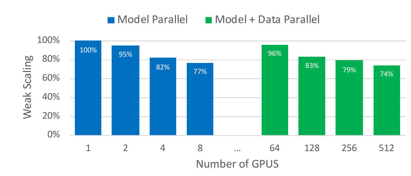
在本节中,我们将展示针对模型和模型+数据并行两种情形、相对于模型参数量的弱扩展。弱扩展通常通过增大批大小来实现,然而这种方法无法解决训练单块 GPU 放不下的大模型的问题,并且在批大小很大时会导致训练收敛性下降。与之相反,我们在这里使用弱扩展来训练原本不可能训练的更大模型。所有扩展数字的基线是表 1 中的第一个配置(12 亿参数)在单块 GPU 上运行。这是一个很强的基线,因为它在整个训练过程中达到 39 TeraFLOPS,是 DGX-2H 服务器中单 GPU 理论峰值 FLOPS 的 30%。
图 5 展示了模型并行和模型+数据并行两种情形的扩展值。我们在两种设置中都观察到了极好的扩展数字。例如,采用 8 路(8 块 GPU)模型并行的 83 亿参数情形达到了线性扩展的 77%。模型+数据并行需要额外通信梯度,因此扩展数字略有下降。然而,即使对于运行在 512 块 GPU 上的最大配置(83 亿参数),相对于强单 GPU 基线配置(12 亿参数)的线性扩展,我们仍达到 74% 的扩展。更多扩展性分析见附录 D。
5.2 GPT-2 语言建模结果 Language Modeling Results Using GPT-2
为了证明大型语言模型能够进一步推进最先进水平,我们考虑训练表 2 中所列规模与配置的 GPT-2 模型。355M 模型在规模和配置上与 BERT-Large 模型(Devlin et al., 2018)相当。2.5B 模型比此前最大的 GPT-2 模型更大,而据我们所知,8.3B 模型比任何已训练过的从左到右 Transformer 语言模型都要大。我们使用第 4 节所述的流程来训练和评估我们的语言模型。表 2 还列出了推进一个 epoch 所需的时间,一个 epoch 相当于 68,507 次迭代。例如,对于 512 块 GPU 上的 8.3B 模型,每个 epoch 约需两天。与表 1 中扩展性研究所用的配置相比,2.5B 模型相同,8.3B 模型的注意力头数为 24 而非 32,而 355M 模型比以往见过的任何模型都小得多,但仍使用 64 块 GPU 训练,因此每个 epoch 的时间要短得多。
| 参数量 Parameter Count |
层数 Layers |
隐藏维度 Hidden Size |
注意力头数 Attn Heads |
每头隐藏维度 Hidden Size per Head |
GPU 总数 Total GPUs |
每个 epoch 用时(天) Time per Epoch (days) |
|---|---|---|---|---|---|---|
| 355M | 24 | 1024 | 16 | 64 | 64 | 0.86 |
| 2.5B | 54 | 1920 | 20 | 96 | 128 | 2.27 |
| 8.3B | 72 | 3072 | 24 | 128 | 512 | 2.10 |
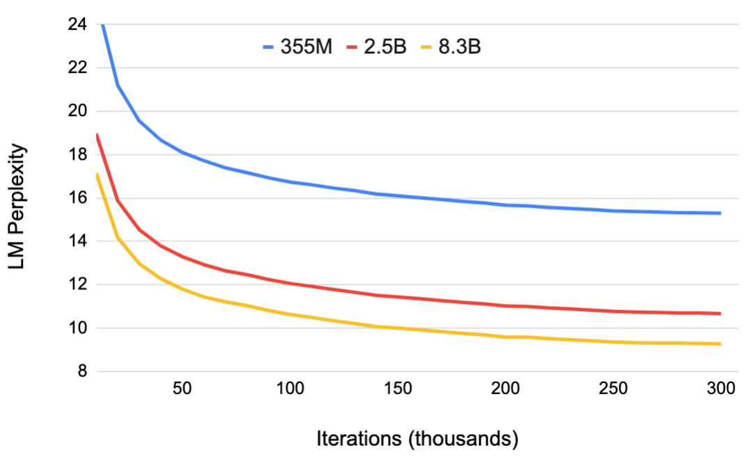
图 6 展示了验证集困惑度随迭代次数的变化。随着模型规模增大,验证困惑度下降,8.3B 模型达到了 9.27 的验证困惑度。我们在表 3 中报告了训练后的模型在 LAMBADA 和 WikiText103 数据集上的零样本(zero-shot)评估结果。关于评估方法的更多细节,请参见附录 E。我们观察到这样的趋势:增大模型规模同样会使 WikiText103 上的困惑度更低,LAMBADA 上的完形填空准确率更高。我们的 8.3B 模型在 WikiText103 测试集上达到了最先进的困惑度,经过适当调整后的困惑度为 10.81。8.3B 模型在 LAMBADA 任务上以 66.51% 的准确率同样超越了此前的完形填空准确率结果。我们在附录 C 中收录了 83 亿参数模型生成的样例。最近,微软与 NVIDIA 合作,使用 Megatron 训练了一个名为 Turing-NLG(Microsoft, 2020)的 170 亿参数 GPT-2 模型,并表明随着模型规模扩大,精度进一步提升,凸显了更大模型的价值。
| 模型 Model |
Wikitext103 困惑度 ↓ Perplexity |
LAMBADA 准确率 ↑ Accuracy |
|---|---|---|
| 355M | 19.31 | 45.18% |
| 2.5B | 12.76 | 61.73% |
| 8.3B | 10.81 | 66.51% |
| 此前 SOTA(Previous SOTA) | 15.79 | 63.24% |
为确保我们没有在测试集中出现的数据上进行训练,我们按照先前工作(Radford et al., 2019)的做法,计算测试集中同时出现在训练集中的 8-gram 的百分比。WikiText103 测试集至多有 10.8% 的重叠,LAMBADA 测试集(Paperno et al., 2016)至多有 1.4% 的重叠。需要指出的是,WikiText103 测试集与 WikiText103 训练集本身就已有 9.09% 的重叠(Radford et al., 2019)。由于这些与先前工作一致,我们有信心没有测试数据中的文档被无意地包含进我们的训练数据。
5.3 BERT 双向 Transformer 结果 Bi-directional Transformer Results Using BERT
在本节中,我们将我们的方法应用于 BERT 风格的 Transformer 模型,并研究模型规模扩展对若干下游任务的影响。先前的工作(Lan et al., 2019)发现,将模型规模增大到超过拥有 336M 参数的 BERT-large 会导致意料之外的模型退化。为了解决这一退化,该工作作者(Lan et al., 2019)引入了参数共享,并表明其模型的扩展性相比原始 BERT 模型要好得多。
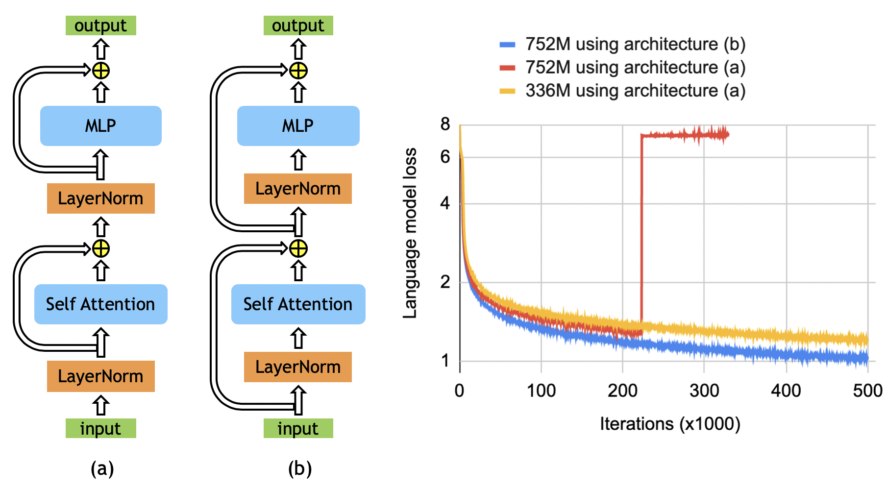
我们进一步研究了这一现象,并通过实验证明,如图 7 所示重新排列 layer normalization 与残差连接的顺序,对于使 BERT 风格模型能够扩展到 BERT-Large 之上至关重要。图 7 中的架构 (b) 消除了使用原始 BERT 架构 (a) 时观察到的不稳定性,并且训练损失也更低。据我们所知,我们是第一个报告这样的改动能够训练更大 BERT 模型的工作。
使用图 7(b) 中的架构改动,我们考虑表 4 所详述的三种情形。336M 模型与 BERT-large 规模相同。1.3B 与 BERT-xlarge 配置相同,该配置此前已被证明比 336M 的 BERT-large 模型得到更差的结果(Lan et al., 2019)。我们进一步通过增大隐藏维度以及增加层数来扩展 BERT 模型,得到 3.9B 参数的情形。在所有情形下,每个注意力头的隐藏维度保持为 64 不变。336M 和 1.3B 模型训练 200 万次迭代,而 3.9B 模型训练了 150 万次迭代,且仍在训练中。在 3% 的留出集上,336M、1.3B 和 3.9B 模型分别达到 1.58、1.30 和 1.16 的验证集困惑度,随模型规模单调下降。我们在若干下游任务上对训练好的模型进行微调,包括 GLUE 基准(Wang et al., 2019)中的 MNLI 和 QQP,Stanford 问答数据集(Rajpurkar et al., 2016; 2018)中的 SQuAD 1.1 和 SQuAD 2.0,以及阅读理解数据集 RACE(Lai et al., 2017)。对于微调,我们遵循与 (Liu et al., 2019b) 相同的流程。我们首先对批大小和学习率进行超参数调优。获得最佳值后,我们报告 5 个不同随机初始化种子上的开发集结果中位数。每个模型和任务所用的超参数在附录 A 中给出。
| 参数量 Parameter Count |
层数 Layers |
隐藏维度 Hidden Size |
注意力头数 Attention Heads |
GPU 总数 Total GPUs |
|---|---|---|---|---|
| 336M | 24 | 1024 | 16 | 128 |
| 1.3B | 24 | 2048 | 32 | 256 |
| 3.9B | 48 | 2560 | 40 | 512 |
表 5 给出了 MNLI、QQP、SQuAD 1.1 和 SQuAD 2.0 的开发集结果以及 RACE 的测试集结果。对于 RACE 的测试集结果,我们先用开发集找到在 5 个随机种子上取得中位数分数的检查点,并报告该检查点在测试集上的结果。我们还报告了 SQuAD 开发集和 RACE 测试集的 5 路集成(ensemble)结果。从表 5 中我们观察到:(a) 随着模型规模增大,所有情形下游任务的性能都得到提升;(b) 与其他基于 BERT 的模型相比,我们的 3.9B 模型在开发集上取得了最先进的结果;(c) 我们的 3.9B 模型在 RACE 测试集上同时取得了单模型和集成的 SOTA 结果。
| 模型 Model |
已训练 token 比例 trained tokens ratio |
MNLI m/mm 准确率 (开发集) |
QQP 准确率 (开发集) |
SQuAD 1.1 F1 / EM (开发集) |
SQuAD 2.0 F1 / EM (开发集) |
RACE m/h 准确率 (测试集) |
|---|---|---|---|---|---|---|
| RoBERTa (Liu et al., 2019b) | 2 | 90.2 / 90.2 | 92.2 | 94.6 / 88.9 | 89.4 / 86.5 | 83.2 (86.5 / 81.8) |
| ALBERT (Lan et al., 2019) | 3 | 90.8 | 92.2 | 94.8 / 89.3 | 90.2 / 87.4 | 86.5 (89.0 / 85.5) |
| XLNet (Yang et al., 2019) | 2 | 90.8 / 90.8 | 92.3 | 95.1 / 89.7 | 90.6 / 87.9 | 85.4 (88.6 / 84.0) |
| Megatron-336M | 1 | 89.7 / 90.0 | 92.3 | 94.2 / 88.0 | 88.1 / 84.8 | 83.0 (86.9 / 81.5) |
| Megatron-1.3B | 1 | 90.9 / 91.0 | 92.6 | 94.9 / 89.1 | 90.2 / 87.1 | 87.3 (90.4 / 86.1) |
| Megatron-3.9B | 1 | 91.4 / 91.4 | 92.7 | 95.5 / 90.0 | 91.2 / 88.5 | 89.5 (91.8 / 88.6) |
| ALBERT ensemble (Lan et al., 2019) | 95.5 / 90.1 | 91.4 / 88.9 | 89.4 (91.2 / 88.6) | |||
| Megatron-3.9B ensemble | 95.8 / 90.5 | 91.7 / 89.0 | 90.9 (93.1 / 90.0) |
6 结论与未来工作 Conclusion and Future Work
在这项工作中,我们仅通过对现有 PyTorch Transformer 实现做少量修改来实现模型并行,成功突破了传统的每个模型占用单块 GPU 的训练所带来的限制。我们在 512 块 NVIDIA V100 GPU 上使用 8 路模型并行,高效地训练了参数量高达 83 亿的基于 Transformer 的模型,并在整个应用上持续达到最高 15.1 PetaFLOPs。我们还表明,对于 BERT 模型,随着模型规模增大,仔细处理类 BERT 模型中 layer normalization 的位置对于获得更高的精度至关重要。我们研究了模型规模对下游任务精度的影响,在下游任务上取得了远为优越的结果,并在 WikiText103、LAMBADA 和 RACE 数据集上创造了新的 SOTA。最后,我们开源了代码,以便未来利用模型并行 Transformer 的工作。
未来工作有若干方向。继续增大预训练规模是一条很有前景的研究路线,将进一步检验现有的深度学习硬件和软件。为实现这一点,需要提升优化器的效率并减小其内存占用。此外,训练参数量超过 160 亿的模型所需的内存将超过一台 DGX-2H 的 16 块 GPU 所能提供的内存。对于这样的模型,结合层内与层间模型并行以及节点间模型并行的混合方式会更合适。另外还有三个值得研究的方向:(a) 预训练不同的模型族(XLNet、T5);(b) 在更困难、更多样的下游任务(例如生成式问答、摘要和对话)上评估大模型的性能;(c) 使用知识蒸馏,从这些大型预训练教师模型训练小型学生模型。
参考文献 References
- Abadi, M., Agarwal, A., Barham, P., Brevdo, E., Chen, Z., Citro, C., Corrado, G. S., Davis, A., Dean, J., Devin, M., Ghemawat, S., Goodfellow, I., Harp, A., Irving, G., Isard, M., Jia, Y., Jozefowicz, R., Kaiser, L., Kudlur, M., Levenberg, J., Mané, D., Monga, R., Moore, S., Murray, D., Olah, C., Schuster, M., Shlens, J., Steiner, B., Sutskever, I., Talwar, K., Tucker, P., Vanhoucke, V., Vasudevan, V., Viégas, F., Vinyals, O., Warden, P., Wattenberg, M., Wicke, M., Yu, Y., and Zheng, X. TensorFlow: Large-scale machine learning on heterogeneous systems, 2015. URL http://tensorflow.org/. Software available from tensorflow.org.
- Ba, J. L., Kiros, J. R., and Hinton, G. E. Layernorm. CoRR, abs/1607.06450, 2016. URL http://arxiv.org/abs/1607.06450.
- Chen, C.-C., Yang, C.-L., and Cheng, H.-Y. Efficient and robust parallel dnn training through model parallelism on multi-gpu platform. arXiv:1809.02839, 2018.
- Chen, T., Xu, B., Zhang, C., and Guestrin, C. Training deep nets with sublinear memory cost. CoRR, abs/1604.06174, 2016. URL http://arxiv.org/abs/1604.06174.
- Dai, Z., Yang, Z., Yang, Y., Carbonell, J. G., Le, Q. V., and Salakhutdinov, R. Transformer-xl: Attentive language models beyond a fixed-length context. CoRR, abs/1901.02860, 2019. URL http://arxiv.org/abs/1901.02860.
- Devlin, J., Chang, M.-W., Lee, K., and Toutanova, K. Bert: Pre-training of deep bidirectional transformers for language understanding, 2018.
- Goyal, P., Dollár, P., Girshick, R. B., Noordhuis, P., Wesolowski, L., Kyrola, A., Tulloch, A., Jia, Y., and He, K. Accurate, large minibatch SGD: training imagenet in 1 hour. CoRR, abs/1706.02677, 2017.
- Harlap, A., Narayanan, D., Phanishayee, A., Seshadri, V., Devanur, N., Ganger, G., and Gibbons, P. Pipedream: Fast and efficient pipeline parallel dnn training. arXiv:1806.03377, 2018.
- Hendrycks, D. and Gimpel, K. Bridging nonlinearities and stochastic regularizers with gaussian error linear units. CoRR, abs/1606.08415, 2016. URL http://arxiv.org/abs/1606.08415.
- Howard, J. and Ruder, S. Fine-tuned language models for text classification. CoRR, abs/1801.06146, 2018.
- Huang, Y., Cheng, Y., Chen, D., Lee, H., Ngiam, J., Le, Q. V., and Chen, Z. Gpipe: Efficient training of giant neural networks using pipeline parallelism. CoRR, abs/1811.06965, 2018. URL http://arxiv.org/abs/1811.06965.
- Jia, Z., Zaharia, M., and Aiken, A. Beyond data and model parallelism for deep neural networks. arXiv:1807.05358, 2018.
- Joshi, M., Chen, D., Liu, Y., Weld, D. S., Zettlemoyer, L., and Levy, O. Spanbert: Improving pre-training by representing and predicting spans. arXiv:1907.10529, 2019.
- Keskar, N. S., Mudigere, D., Nocedal, J., Smelyanskiy, M., and Tang, P. T. P. On large-batch training for deep learning: Generalization gap and sharp minima. ICLR, 2017.
- Khandelwal, U., Levy, O., Jurafsky, D., Zettlemoyer, L., and Lewis, M. Generalization through memorization: Nearest neighbor language models. arXiv:1911.00172, 2019.
- Kingma, D. P. and Ba, J. Adam: A method for stochastic optimization. arXiv preprint arXiv:1412.6980, 2014.
- Lai, G., Xie, Q., Liu, H., Yang, Y., and Hovy, E. Race: Large-scale reading comprehension dataset from examinations. arXiv:1704.04683, 2017.
- Lan, Z., Chen, M., Goodman, S., Gimpel, K., and Soricut, P. S. R. Albert: A lite bert for self-supervised learning of language representations. arXiv:1909.11942, 2019.
- Li, M., Andersen, D. G., Park, J. W., Smola, A. J., Ahmed, A., Josifovski, V., Long, J., Shekita, E. J., and Su, B.-Y. Scaling distributed machine learning with the parameter server, 2014.
- Liu, X., He, P., Chen, W., and Gao, J. Multi-task deep neural networks for natural language understanding. CoRR, abs/1901.11504, 2019a. URL http://arxiv.org/abs/1901.11504.
- Liu, Y., Ott, M., Goyal, N., Du, J., Joshi, M., Chen, D., Levy, O., Lewis, M., Zettlemoyer, L., and Stoyanov, V. Roberta: A robustly optimized BERT pretraining approach. CoRR, abs/1907.11692, 2019b. URL http://arxiv.org/abs/1907.11692.
- Loshchilov, I. and Hutter, F. Decoupled weight decay regularization. In International Conference on Learning Representations, 2019. URL https://openreview.net/forum?id=Bkg6RiCqY7.
- McCann, B., Bradbury, J., Xiong, C., and Socher, R. Learned in translation: Contextualized word vectors. CoRR, abs/1708.00107, 2017.
- Melamud, O., Goldberger, J., and Dagan, I. context2vec: Learning generic context embedding with bidirectional lstm. In Proceedings of The 20th SIGNLL Conference on Computational Natural Language Learning, pp. 51–61, 01 2016.
- Merity, S., Xiong, C., Bradbury, J., and Socher, R. Pointer sentinel mixture models. CoRR, abs/1609.07843, 2016. URL http://arxiv.org/abs/1609.07843.
- Micikevicius, P., Narang, S., Alben, J., Diamos, G. F., Elsen, E., Garcia, D., Ginsburg, B., Houston, M., Kuchaiev, O., Venkatesh, G., and Wu, H. Mixed precision training. CoRR, abs/1710.03740, 2017.
- Microsoft. Turing-nlg: A 17-billion-parameter language model by microsoft, 2020. URL https://www.microsoft.com/en-us/research/blog/turing-nlg-a-17-billion-parameter-language-model-by-microsoft/.
- Mikolov, T., Deoras, A., Kombrink, S., Burget, L., and Černocký, J. Empirical evaluation and combination of advanced language modeling techniques. In Twelfth Annual Conference of the International Speech Communication Association, 2011.
- Mikolov, T., Sutskever, I., Chen, K., Corrado, G., and Dean, J. Distributed representations of words and phrases and their compositionality. CoRR, abs/1310.4546, 2013.
- NVIDIA. Mixed precision training: Choosing a scaling factor, 2018. URL https://docs.nvidia.com/deeplearning/sdk/mixed-precision-training/index.html#scalefactor.
- Paperno, D., Kruszewski, G., Lazaridou, A., Pham, Q. N., Bernardi, R., Pezzelle, S., Baroni, M., Boleda, G., and Fernández, R. The LAMBADA dataset: Word prediction requiring a broad discourse context. CoRR, abs/1606.06031, 2016. URL http://arxiv.org/abs/1606.06031.
- Pennington, J., Socher, R., and Manning, C. D. Glove: Global vectors for word representation, 2014. URL https://www.aclweb.org/anthology/D14-1162.
- Peters, M. E., Neumann, M., Iyyer, M., Gardner, M., Clark, C., Lee, K., and Zettlemoyer, L. Deep contextualized word representations. CoRR, abs/1802.05365, 2018. URL http://arxiv.org/abs/1802.05365.
- Radford, A., Józefowicz, R., and Sutskever, I. Learning to generate reviews and discovering sentiment. CoRR, abs/1704.01444, 2017.
- Radford, A., Narasimhan, K., Salimans, T., and Sutskever, I. Improving language understanding by generative pre-training, 2018. URL https://blog.openai.com/language-unsupervised/.
- Radford, A., Wu, J., Child, R., Luan, D., Amodei, D., and Sutskever, I. Better language models and their implications, 2019. URL https://openai.com/blog/better-language-models/.
- Raffel, C., Shazeer, N., Roberts, A., Lee, K., Narang, S., Matena, M., Zhou, Y., Li, W., and Liu, P. J. Exploring the limits of transfer learning with a unified text-to-text transformer. arXiv:1910.10683, 2019.
- Rajpurkar, P., Zhang, J., Lopyrev, K., and Liang, P. Squad: 100,000+ questions for machine comprehension of text. EMNLP, 2016.
- Rajpurkar, P., Jia, R., and Liang, P. Know what you don't know: Unanswerable questions for squad. ACL, 2018.
- Ramachandran, P., Liu, P. J., and Le, Q. V. Unsupervised pretraining for sequence to sequence learning. CoRR, abs/1611.02683, 2016. URL http://arxiv.org/abs/1611.02683.
- Shazeer, N., Cheng, Y., Parmar, N., Tran, D., Vaswani, A., Koanantakool, P., Hawkins, P., Lee, H., Hong, M., Young, C., Sepassi, R., and Hechtman, B. Mesh-TensorFlow: Deep learning for supercomputers. In Neural Information Processing Systems, 2018.
- Trinh, T. H. and Le, Q. V. A simple method for commonsense reasoning. CoRR, abs/1806.02847, 2018. URL http://arxiv.org/abs/1806.02847.
- Turian, J., Ratinov, L., and Bengio, Y. Word representations: A simple and general method for semi-supervised learning. In Proceedings of the 48th Annual Meeting of the Association for Computational Linguistics, ACL '10, pp. 384–394, Stroudsburg, PA, USA, 2010. Association for Computational Linguistics.
- Valiant, L. G. A bridging model for parallel computation. Communications of the ACM, 33(8):103-111, 1990.
- Vaswani, A., Shazeer, N., Parmar, N., Uszkoreit, J., Jones, L., Gomez, A. N., Kaiser, L., and Polosukhin, I. Attention is all you need. CoRR, abs/1706.03762, 2017.
- Wang, A., Singh, A., Michael, J., Hill, F., Levy, O., and Bowman, S. R. Glue: A multi-task benchmark and analysis platform for natural language understanding. ICLR, 2019.
- Yang, Z., Dai, Z., Yang, Y., Carbonell, J. G., Salakhutdinov, R., and Le, Q. V. Xlnet: Generalized autoregressive pretraining for language understanding. CoRR, abs/1906.08237, 2019. URL http://arxiv.org/abs/1906.08237.
- You, Y., Gitman, I., and Ginsburg, B. Large batch training of convolutional networks. arXiv:1708.03888, 2017.
- You, Y., Li, J., Reddi, S., Hseu, J., Kumar, S., Bhojanapalli, S., Song, X., Demmel, J., and Hsieh, C.-J. Large batch optimization for deep learning: Training bert in 76 minutes. arXiv:1904.00962, 2019.
- Zellers, R., Holtzman, A., Rashkin, H., Bisk, Y., Farhadi, A., Roesner, F., and Choi, Y. Defending against neural fake news. CoRR, abs/1905.12616, 2019. URL http://arxiv.org/abs/1905.12616.
- Zhu, Y., Kiros, R., Zemel, R. S., Salakhutdinov, R., Urtasun, R., Torralba, A., and Fidler, S. Aligning books and movies: Towards story-like visual explanations by watching movies and reading books. CoRR, abs/1506.06724, 2015.
附录 A BERT 微调超参数 BERT Finetuning Hyperparameters
表 6 给出了微调期间每个模型和任务所用的超参数。
| 任务 Task |
模型 Model |
批大小 Batch size |
学习率 Learning rate |
训练轮数 Training epochs |
|---|---|---|---|---|
| MNLI | 336M | 128 | 1e-5 | 10 |
| 1.3B | ||||
| 3.8B | ||||
| QQP | 336M | 128 | 5e-5 | 12 |
| 1.3B | 128 | 3e-5 | ||
| 3.8B | 256 | 4e-5 | ||
| SQUAD 1.1 | 336M | 64 | 3e-5 | 2 |
| 1.3B | 48 | 3e-5 | ||
| 3.8B | 48 | 1e-5 | ||
| SQUAD 2.0 | 336M | 48 | 3e-5 | 2 |
| 1.3B | 64 | 3e-5 | ||
| 3.8B | 48 | 1e-5 | ||
| RACE | 336M | 32 | 2e-5 | 3 |
| 1.3B | 16 | 1e-5 | ||
| 3.8B | 32 | 2e-5 |
附录 B 模型并行补充材料 Model Parallel Supplementary Material
在本节中,我们给出混合模型并行与数据并行以及随机数生成处理的更多细节。
B.1 混合模型并行与数据并行 Hybrid Model and Data Parallelism
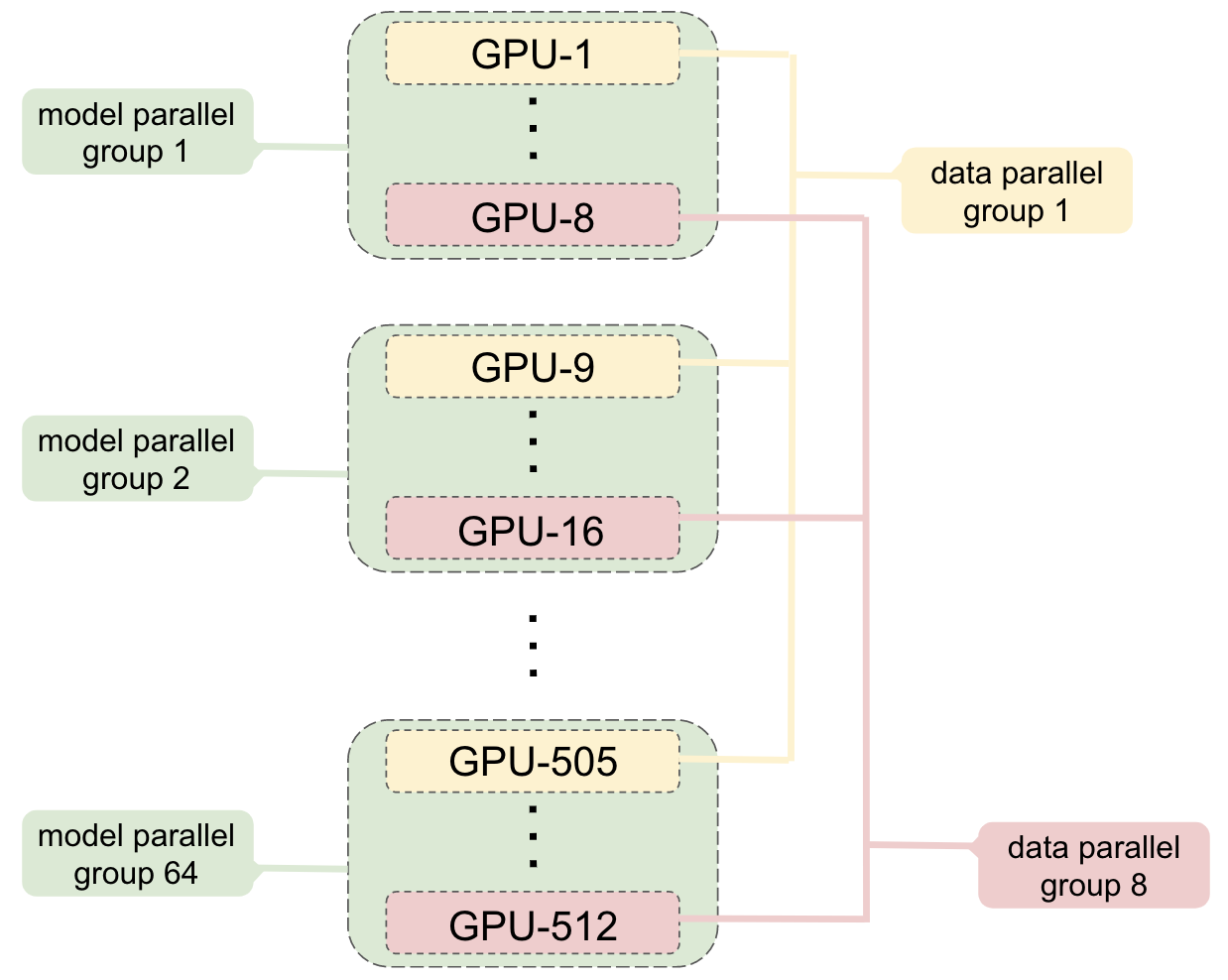
模型并行与数据并行是正交的,因此我们可以同时使用二者,在合理的时间内训练大型模型。图 8 展示了用于混合模型并行与数据并行的 GPU 分组。同一服务器内的两块或更多 GPU 组成模型并行组(例如图 8 中的 GPU 1 到 8),并包含分布在这些 GPU 上的一份模型实例。其余 GPU(可能在同一服务器内,但更常见的是位于其他服务器)运行额外的模型并行组。每个模型并行组中处于相同位置的 GPU(例如图 8 中的 GPU 1、9、……、505)构成数据并行组,使得一个数据并行组内的所有 GPU 持有相同的模型参数。在反向传播期间,我们并行运行多个梯度 all-reduce 操作,对每个不同的数据并行组内的权重梯度进行规约。所需 GPU 的总数是模型并行组数与数据并行组数的乘积。例如,对于 83 亿参数的模型,我们每个模型并行组使用 8 块 GPU 并采用 64 路数据并行,总共 512 块 GPU。所有通信都在 PyTorch 中通过 Python 调用 NCCL 实现。每个模型并行组内的 GPU 在组内所有 GPU 之间执行 all-reduce。对于数据并行,每个 all-reduce 操作都在每个模型并行组各取一块 GPU 的范围内进行。
B.2 模型并行中的随机数生成 Model Parallel Random Number Generation
使用随机数生成的技术(例如 dropout)是现代深度学习训练的主要内容。Transformer 在残差连接之前的模型并行区域之外有 dropout 层,在自注意力块的模型并行区域之内也有 dropout 层。由于一些 dropout 层处于模型并行区域,而另一些不在,我们需要谨慎处理随机数生成,以确保 dropout 正确工作。为了在模型并行 worker 之间同步残差连接的 dropout,我们在训练开始时用相同的种子为随机数生成器设定种子。这使得所有模型并行 worker 上的 dropout 模式相同。然而,模型并行区域内的 dropout 应该在各个 worker 上产生不同的随机模式,以便在整个操作范围内实现随机性。为此,我们为模型并行区域内的 dropout 维护一个单独的随机数生成器。该随机数生成器为每个模型并行 worker 使用唯一的种子。
附录 C 文本样例 Text Samples
下面是 Megatron-LM 使用上下文提示(context prompt)生成的一些文本样例,其中部分文本被截断。
说明:以下样例是模型生成的文本,按原文保留英文,不作翻译。其中 “Context” 为给定的提示文本,“Megatron-LM” 之后为模型生成的续写。
Context: There is a major force uniting Americas fiercely partisan politicians: big technology companies. Democrats and Republicans at the federal and state levels are coming together to scrutinize the power of the Silicon Valley giants and, potentially, to rein them in. Letitia James, the Democratic attorney general of New York, announced on Friday that attorneys general in eight states four Democrats and four Republicans and the District of Columbia had begun an antitrust investigation of Facebook.
Megatron-LM: The probe, which Ms. James said was likely to result in a lawsuit, is the latest in a string of high-profile regulatory actions, in state and federal courts, that challenge the market dominance of tech companies. The Justice Department is also investigating Facebook's data practices and whether the company violated a 2011 consent decree with the Federal Trade Commission that required the company to obtain explicit consent from users before sharing their personal information with third parties.
What might prompt a bipartisan coalition to sue Facebook? It isn't clear that there's any one thing. But lawmakers and regulators have been increasingly alarmed by the company's recent controversies, which include a data breach affecting more than 50 million users, the spread of fake news on the platform, and the spreading of propaganda by Russian-backed accounts during the 2016 election.
It's also not clear how serious the Democratic attorneys general are about filing a lawsuit. While the attorneys general announced their investigation in a press release, they said they had not yet reached a decision on whether to sue. In the past, some of the attorneys general have focused their efforts on trying to extract settlements from the tech companies without filing lawsuits.
"As attorneys general who have investigated and prosecuted health-care fraud, price-fixing, and other violations of our states' antitrust laws, we are committed to holding companies accountable when they fail to protect consumers and competition in the market," Ms. James said in a statement.
The investigation, which was first reported by The New York Times, was announced as the companies that dominate the tech industry are facing scrutiny from antitrust regulators around the world. Google, Twitter, Facebook and Amazon have faced a series of antitrust probes and class-action lawsuits in the United States and Europe ...
Context: A flower, sometimes known as a bloom or blossom, is the reproductive structure found in flowering plants (plants of the division Magnoliophyta, also called angiosperms). The biological function of a flower is to effect reproduction, usually by providing a mechanism for the union of sperm with eggs.
Megatron-LM: The structural components of the flower are the petals and sepals, which are the reproductive organs, the hypanthium, which forms the base of the flower, and the calyx, which is the stigma. A flower is a composite structure, made up of sepals and petals, the sepals being composed of three fused tepals and the petals of two fused petals, though there are a few exceptions to this rule. The three sepals are fused to form a tube called the calyx, which is the structure that attracts the pollinating insects. The petals are composed of two fused sepals (the outer ones) which open and fold inward (clasp) at the tips, forming the petals. The four sepals and petals are united to form a corolla, the outermost structure of a flower that carries pollen.
The structure of the flower has important functional significance, including protection of the ovary from insects and the transfer of pollen between the male and female parts of a flower. The structure of the flower is also used by the plants to attract pollinators, for example by the shape of the petals and the colours of the stamens.
The structure of a flower varies widely between plants. The simplest flowers are unbranched and made up of only two sepals and a single petal. Other examples are composed of several petals joined together, with the innermost sepals completely fused to form a tube called the calyx. The petals are usually coloured to attract insects, which can only see certain wavelengths of light. The sepals are often coloured too, but usually have a more limited range of colours.
Some flowers have additional structures, such as stamens, anthers and ovaries. The presence of stamens and anthers in some flowers is used for cross-pollination. The ovary is the organ where the female gametes are produced, and is the first structure that is developed in an embryo of a flower. The ovary is the female flower's reproductive system, and consists of the ovary wall, the ovule, and the oviduct.
Flowers vary in their size and shape, from tiny to huge, and are often brightly coloured. Flowers may be seen as part of a larger structure, such as a flower head, an inflorescence, a bract, a spathe, or a carpels.
The term "flower" is usually applied to the floral structures that are visible externally, but many ...
Context: OpenAI did not release the full GPT-2 model due to concerns of malicious use, but they did release a smaller version equivalent in size to the original GPT (117 M parameters), trained on the new, larger dataset. Although not as powerful as the large model, the smaller version still has some language generation chops.
Megatron-LM: In December 2016, DeepMind released an even larger model, GPT-3, with more than 1.5 billion parameters. DeepMind has no plans to release the model, so the question remains whether other AI researchers will be able to copy and build on it.
Other language models have been built using other techniques. In 2016, a team of researchers at Columbia University, the University of Toronto, and Google DeepMind showed that neural network-based models, including deep neural networks, can learn the grammatical rules of a language. A group at Google DeepMind demonstrated that these rules could be represented in a network as a kind of decision tree, where the nodes in the tree are the words in the sentence, and the rules for the words are represented by the decision nodes at the end of the tree. The network would go through the network in order to choose the next word in the sentence based on whether it follows the rules or not. In 2017, the team at DeepMind released a paper detailing the training and performance of their model.
The problems with the model are many. One of the biggest issues is that grammatical rules are ambiguous. For example, the phrase "I came down" could mean I came down from the stairs, or I came down from the sky. In English, there are numerous other examples of sentences that are ambiguous. The model does not have any way to tell the difference between the ambiguous sentences, and so it simply makes a prediction about the entire sentence based on what rules it does know. This makes the model vulnerable to the phenomenon of overfitting. In order to avoid this, models must be trained using a large set of data, so that the model can find useful patterns in the data, and use those patterns to help make predictions. This approach is also prone to errors, as it relies on the training data to help make correct predictions, and the data might be incorrectly labeled, resulting in a model that produces a poor set of predictions. In the case of GPT-2, the model only has about 100 training sentences for each type of phrase (subject-verb-object).
Additionally, languages have different rules for different types of phrasing. In English, the subject-verb-object construction is fairly universal, but other languages have different rules, which makes training a GPT more complicated.
Finally, there is an inherent trade-off between the number of rules and the performance of the model ...
Context: The 36th International Conference on Machine Learning (ICML 2019) will be held in Long Beach, CA, USA from June 10th to June 15th, 2019. The conference will consist of one day of tutorials (June 10), followed by three days of main conference sessions (June 11-13), followed by two days of workshops (June 14-15).
Megatron-LM: With a broad scope, the conference addresses the challenges and opportunities in machine learning for practitioners and researchers. The conference program will feature sessions that cover different machine learning topics, from reinforcement learning to computational biology and from AI to deep learning. It is the world's premier forum for exploring and presenting advances in machine learning.
ICML 2019 will offer an impressive range of sessions, which will be of interest to practitioners, researchers, and students. Some of the topics we will cover include:
- Reinforcement learning
- Soft Computing
- Computational biology
- Convolutional networks
- Deep learning
- Statistical learning theory
- Statistical learning machine
- Natural language processing
- Biology
- Awards
Since its first edition, the conference has grown and evolved. Today, it is the premier forum for showcasing state-of-the-art research in machine learning. The conference is widely recognized as the preeminent venue for showcasing the latest research in machine learning, and a place where practitioners, researchers, and students can exchange ideas and insights.
The conference is a peer-reviewed venue that draws its prestige and influence from the excellence of the presentations and the quality of the invited speakers. With over 50% of all talks selected based on their content by an expert committee, it is clear that the conference's high standards of research and quality keep a very high bar.
Context: Rescue workers on Tuesday found a flight recorder from the Russian plane that crashed into the Black Sea over the weekend, the defense ministry said. All 92 people aboard the Russian military's Tu-154 plane are believed to have died Sunday morning when it crashed two minutes after taking off from the southern Russian city of Sochi.
Megatron-LM: A child holds up a portrait of a dead relative at a makeshift morgue in a building belonging to a local government in the town of Petropavlovsk-Kamchatsky. A Russian Defense Ministry Tu-154 plane with 92 people on board crashed into the Black Sea on Sunday morning shortly after taking off from the southern Russian city of Sochi. (Yuri Kochetkov/EPA)
According to the ministry, the plane was found at a depth of more than 1,000 feet and the recorder was damaged. "The defense ministry has decided to hand over the recorder to the Interstate Aviation Committee, which is the main investigative body in the air crash," the statement said.
The search for the plane's black boxes is being hampered by strong winds and rough seas. Investigators have launched a criminal probe into the crash, which officials said was likely caused by a technical fault.
Russian President Vladimir Putin declared Wednesday a day of mourning for the victims.
附录 D 进一步的扩展性分析 Further Scaling Analysis
在本节中,我们研究注意力头数对扩展结果的影响。我们还给出 12 亿参数模型的强扩展结果。
D.1 注意力头数与扩展性 Attention Heads and Scaling
本节研究注意力头数对模型并行扩展的影响。为此,我们考虑 83 亿参数、8 路模型并行的配置,并将头数从 16 变化到 32。结果见表 7。随着注意力头数增加,自注意力层内的一些 GEMM 变小,且自注意力 softmax 中的元素数量增加。这会导致扩展效率略有下降。未来的研究应当对这一超参数保持谨慎,以设计能在模型速度与模型精度之间取得平衡的大型 Transformer 模型。
| 注意力头数 Attention heads |
每头隐藏维度 Hidden size per head |
扩展效率 Scaling Efficiency |
|---|---|---|
| 16 | 192 | 82% |
| 24 | 128 | 80% |
| 32 | 96 | 77% |
D.2 强扩展 Strong Scaling
我们的模型并行主要是为了训练无法放入单块 GPU 内存的更大模型而设计的,但它也可以在不增大批大小的情况下加速较小模型的训练。为了测量这种加速,我们训练一个固定为 12 亿参数的模型。我们使用每次迭代固定 8 个样本的批大小,并通过模型并行增加 GPU 数量。结果列于表 8。使用两块 GPU 使训练快 64%。超过这一点后,我们看到收益递减,因为每块 GPU 上的计算量减少,内存带宽和通信开销开始占主导。
| GPU 数量 # of GPUs |
1 | 2 | 4 | 8 |
|---|---|---|---|---|
| 加速比(Speedup) | 1.0 | 1.64 | 2.34 | 2.98 |
附录 E 用 WikiText103 与 LAMBADA 评估语言模型 Evaluating Language Models Using WikiText103 and LAMBADA
在本节中,我们详述在 WikiText103 数据集(Merity et al., 2016)上的评估方法,以及在 LAMBADA 数据集(Paperno et al., 2016)上的完形填空式预测准确率的评估方法。
E.1 Wikitext103 困惑度 Wikitext103 Perplexity
自该基准数据集创建以来的过去几年里,WikiText103 困惑度一直是一个被充分研究的评估标准。困惑度是语料平均交叉熵的指数(Mikolov et al., 2011)。这使其成为表示整句或整篇文本上概率分布的语言模型的自然评估指标。
$$PPL = \exp\!\left(-\frac{1}{T_o}\sum_{t}^{T}\log P(t\,|\,0:t-1)\right) \tag{4}$$为了计算 (4) 中的困惑度,我们按照自己的子词词表对 WikiText103 测试语料进行分词,并对每个 token $[0, T]$ 的交叉熵损失求和。然后,我们用原始分词方案中的 token 数 $T_o$ 对交叉熵损失进行归一化。WikiText103 测试语料本身已经预先按词级别 token 分好词,先前的工作使用这些词级别 token 来计算困惑度。为了在与先前工作相同的起点上评估我们模型的困惑度,我们必须按原始 token 数 $T_o$ 进行归一化,而不是按实际输入模型的分词后数据中的 token 数 $T$。这种预分词还会引入我们训练数据中不存在的文本伪影。为缓解这种分布不匹配,我们先用可逆的反分词器(invertible detokenizers)对 WikiText103 测试数据集进行预处理,以去除与标点和空白相关的各种伪影。$T_o$ 的值是在这一预处理之前计算的。对于 WikiText103 的测试集,$T_o = 245566$,$T = 270329$。
我们还必须对困惑度的计算做一个 Transformer 特有的修改。与基于 RNN 的语言模型不同,Transformer 在固定大小的窗口输入上运行。因此它们无法完整计算 $P(t\,|\,0:t-1)$,只能计算 $P(t\,|\,t-w:t-1)$,其中 $w$ 是我们的上下文大小:1024 个 token。然而,对数据集中每个 token 计算这个值的代价高得令人望而却步,因为我们必须对大小为 $w$ 的上下文进行大约 $T$ 次评估。为了高效评估我们的模型,我们采用一种折中的方法,称为重叠评估(overlapping evaluation):每次将滑动窗口前进某个重叠量 $o$,并且只计算窗口中最后 $o$ 个 token 对应的交叉熵损失。在我们的实验中,我们使用的重叠量为 $o = 32$,并以这种方式在所有滑动窗口上计算损失。
E.2 LAMBADA 完形填空准确率 LAMBADA Cloze Accuracy
处理长程上下文的能力对最先进的语言模型至关重要,也是长文本生成和基于文档的问答等问题的必要前提。像 LAMBADA 这样的完形填空式数据集旨在衡量模型在这类长程上下文中运行和推理的能力。完形填空式阅读理解使用由词 token 组成的上下文 $x = x_{1:t}$,其中一个 token $x_j$ 被掩盖;模型的目标是正确预测缺失的第 $j$ 个 token 的值。为了准确预测缺失的 token,模型需要深入理解周围的上下文,以及语言在这样的上下文中应如何使用。LAMBADA 使用完形填空式阅读理解来测试生成式从左到右语言模型,其构造方式是:取 4–5 句话组成的样例,并将上下文中的最后一个词 $x_t$ 掩盖。我们的模型使用子词单元,因此在 LAMBADA 评估中,我们使用原始的、未经处理的 LAMBADA 数据集,并要求模型预测构成该词 token 的多个子词 token。我们使用 teacher forcing,并且仅当所有输出预测都正确时才认为答案正确。这种表述等价于原始的词 token 预测任务。